
Cumulative Frequency Diagrams
Cumulative Frequency Diagrams are very closely related to Frequency Polygons. They both provide a way of displaying univariate grouped data. Note that you may be required to produce frequency polygons/cumulative frequency diagrams for a given dataset but you may also be asked to do it for a dataset that you are already familiar with. See more on this.
Frequency Polygons
 Frequency Polygons are a common form of chart used for presenting continuous grouped data. Frequencies are plotted on the graph as points (or crosses etc.) and joined up by straight lines. They are called frequency polygons because polygons are shapes where the vertices are joined up by straight lines. However, the first and final points are not joined up so it should be thought of as more of an open shape. The polygon should never touch the bottom axis (unless the data point is 0). See more on Frequency Polygons.
You may be asked to add a Frequency Polygon to a Histogram. See Histograms Example 1.
Cumulative Frequency Diagrams
 ‘Cumulative’ is the adjective for accumulate. It means to add up successively. It follows that cumulative frequency is where the grouped frequencies are added up at each step. Cumulative Frequency Diagrams look very similar to Frequency Polygons but since frequency is added up each time, the graph should trend upwards. Note that for a frequency polygon, the points align with the middle of the interval. For a cumulative frequency diagram, the points align with the end of the intervals. Cumulative frequency diagrams always start from the x-axis.
The lower quartile, the median and the upper quartile can be estimated from a cumulative frequency table and diagram. See the example below for a demonstration.
Frequency Polygons and Cumulative Frequency Diagrams are useful for finding estimates for the quartiles and percentiles but are not so good at showing the ‘spread’ of the data (see Measures of Variation). Box Plots and Histograms are good for this. See the example in Box Plots for more information.
Examples
The following histogram shows the masses of some domestic housecats in kilograms (see more on histograms):

Add the associated frequency polygon to this histogram.
Solution:

Note that the points on the frequency polygon are in the middle of the intervals.
The following table shows the prices in millions of pounds of some houses in a given postcode:
| House Price, P (£m) | Frequency |
 | 21 |
 | 37 |
 | 24 |
 | 11 |
 | 7 |
- Create a cumulative frequency diagram to show this data.
- Find an estimate for the median, the interquartile range and the 10th to 90th percentile range for house prices in this area.
- Show this data in a box plot.
Solution:
- In order to construct a cumulative frequency diagram, it helps to add a column to the table titled ‘Cumulative Frequency’:
House Price, P (£m) Frequency Cumulative Frequency 
21 21 37 58 
24 82 
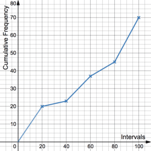
11 93 7 100 The cumulative frequency diagram can be constructed using the cumulative totals. Note the location of the crosses – they align with the end of each interval. The diagram also starts from vertical 0.

- Estimates for the median (red line), Q1 and Q3 (green lines) and the 10th and 90th percentiles (purple lines) can be obtained from the cumulative frequency diagram. The median, for example, is estimated by first locating 50 on the frequency axis, drawing a line across to the cumulative frequency graph and then down onto the house price axis. Similarly, Q1 and Q3 are found from frequencies of 25 and 75. The 10th and 90th percentiles are found from frequencies of 10 and 90. This is because the total frequency is 100. For other frequencies, appropriate proportional adjustments should be made. See more on Quartiles. The estimates can be seen from the graph and give the following:
Median (Q2)= £375,000
IQR (Q3-Q1)= £470,000-£310,000=£160,000
90th – 10th= £575,000-£250,000=£325,000 - From above, Q1=0.31, Q2=0.375 and Q3=0.47 in millions of pounds. In addition, there are no apparent outliers and the minimum and maximum values can be taken as 0.2 and 0.7. The following shows this information in a box plot:


See more on box plots.
Click here for more statistical analysis using this example (Ranges – Example 2).