Locating Roots

Recall that locating roots of a curve means to find the $x$ -coordinates of the points at which the curve crosses the $x$ -axis. To do this analytically means to do it by solving equations using algebra. We know how to find roots analytically for some functions, like quadratics, for example. That is, by solving $y=ax^2+bx+c=0$ for $x$ . We can also do it for some cubics and some trigonometric equations etc. However, there are many equations where we cannot find roots analytically and we must do it numerically. This is where we make ‘guesses’ for the roots and improve them successively via some calculation. This is sometimes known as iteration.

Change of Sign

We can make a first guess at a root of the equation $y=f(x)$ (where $f(x)=0$ cannot be solved analytically) if we see a change in sign of $f(x)$ between two given $x$ -values. For example, consider the graph of $f(x)=\sin(e^x)$ – we cannot find the roots analytically. We can see from the graph that $f(1)=0.4108$ and $f(1.5)=-0.9735$ (using radians). It follows that since $f(1)>0$ and $f(1.5)<0$ , the curve has a root between $x=1$ and $x=1.5$ . Similarly, $f(1.5)<0$ and $f(2)>0$ , the curve has a root between $x=1.5$ and $x=2$ . See Example 1 for successive interval narrowing to get an approximation to the root.

This curve also illustrates some situations to be aware of. Note that $f(0.5)>0$ and $f(1)>0$ and there is no root between $x=0.5$ and $x=1$ . However, $f(1)>0$ and $f(2)>0$ and there are two roots. Hence, it is possible that if the curve has the same sign at two points, there could be no roots or an even number of roots. There are 4 roots between $x=1.5$ and $x=2.9$ , two $x$ -values where the curve is negative. Similarly, $f(2.9)<0$ and $f(3)>0$ and there is one root between $x=2.9$ and $x=3$ . Whereas, $f(2.5)<0$ and $f(3)>0$ and there are three roots between $x=2.5$ and $x=3$ . Hence, it is possible if the curve has different signs at two points, there could be an odd number of roots in between.

These examples illustrate the importance of choosing intervals sufficiently small to indicate the presence of a single root. The final situation to be aware of is the case where a curve has different signs at two points and has no roots in between. This can happen if the curve is not continuous – see some discontinuous curves. In these cases, a change of sign may be due to an asymptote rather than a root.

To summarise: if the function $f(x)$ is continuous on a sufficiently small interval $[a,b]$ , and $f(a)$ and $f(b)$ have opposite signs, then $f(x)$ has a root on the interval $[a,b]$ .

Iteration – Recursive Formula

An alternative way to find roots is to rewrite the equation $f(x)=0$ in the form $x=g(x)$ . Finding the root $x$ that satisfies $f(x)=0$ is then the same as finding the $x$ that satisfies the equation $x=g(x)$ . On a graph, this is the point where the curve of $y=g(x)$ crosses the straight line $y=x$ . By setting up the recursive formula $x_{n+1}=g(x_n)$ , the solution can be found iteratively. This means that we choose $x_0$ and by setting $n=1$ , this formula says that $x_1=g(x_0)$ . So, our next guess for the root is $x_1$ . Similarly, the next guess is $x_2$ , found by setting $n=1$ and evaluating $g(x_1)$ . Recursively, $x_3=g(x_2)$ and $x_4=g(x_3)$ are our next guesses for the root and so on. By choosing a value for $x_0$ well, this formula may converge to a root in one of two ways.

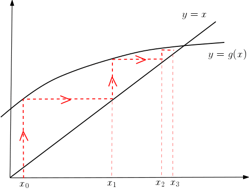
This is an example of a staircase diagram. We put the first choice of $x_0$ into $g(x)$ to find $x_1$ . This is our next choice to put in to $g(x)$ so we go along horizontally to the line $y=x$ so we can put this value in. We move vertically up to find $g(x_1)$ and so on, converging to the solution of $x=g(x)$ , that is the original root, iteratively.

This is an example of a cobweb diagram. As before, we move vertically to find $g(x)$ values and horizontally to find the new corresponding $x$ -values. Due to the shape of the curve, the convergence occurs by going around the solution creating a cobweb-like effect as opposed to the staircase effect seen in the other diagram.

In the above diagrams, the choice of $x_0$ does not affect the convergence. That is, all choices of $x_0$ result in staircase/cobweb convergence towards the root. This is dependent on the shape of the curve when compared with the straight line, however. The diagrams below show how the curve and the choice of $x_0$ can result in staircase/cobweb divergence.

Note that there may be several choices for rewriting $f(x)=0$ in the form $x=g(x)$ when finding the recursive formula $x_{n+1}=g(x_n)$ . The choice of $g(x_n)$ , as well as the choice of $x_0$ , may affect the convergence of the iteration. See Example 2. Even when the sequence converges, the location of the root needs to be justified – see Example 2 for this too.

Locating Roots using the Newton-Raphson Method

The Newton-Raphson method is also an iterative procedure for locating roots. To solve $f(x)=0$ , Newton-Raphson uses a specific recursive formula:

$x_{n+1}=x_n-\frac{f(x_n)}{f'(x_n)}$

Notice the difference between this formula, that uses the derivative $f'(x)$ , as opposed to any $g(x)$ in the iterations above. We revert to looking for the actual root as opposed to the intersection between two curves. To do this, the Newton-Raphson method works using tangents – root guesses are updated by finding where successive tangents cross the $x$ -axis.

The Newton-Raphson formula is essentially a rearrangement of the formula for a derivative. Consider the tangent at $x_0$ , for example. We find the gradient of the tangent (or derivative of the curve) using rise over run: $f'(x_0)=\frac{f(x_0)-0}{x_1-x_0}$ . We can rearrange this to get $x_1=x_0-\frac{f(x_0)}{f'(x_0)}$ . This basically says that we improve the guess for the root by moving backwards by an amount that is the run. If the gradient is rise over run then the run is rise over gradient. See Example 3 for the use of Newton-Raphson in a modelling example where we locate a stationary point rather than a root.

Since there is division by the derivative, the Newton-Raphson method can fail when the derivative is 0. That is, locating roots near a stationary point. This makes sense when considering that a tangent at a stationary points is flat and doesn’t cross the $x$ -axis. We are then unable to use Newton-Raphson to update the root guess. It follows that choosing $x_0$ at a stationary point will result in the method failing. In the case where $f'(x)$ is small, division by a small number creates a large update to the root guess and convergence can be slow. Hence, the choice of $x_0$ should be made away from any stationary points.

Examples

Use successive interval narrowing to find the root of $f(x)=\sin(e^x)$ that is between $x=1$ and $x=1.5$ to 2 decimal places. (Make sure you are using radians).

Solution:

We calculate the function at $x=1.1$ : $f(1.1)=\sin(e^{1.1})=0.13699$ to 5 decimal places. Then at $x=1.2$ : $f(1.2)=\sin(e^{1.2})=-0.17758$ to 5 decimal places. Hence, the root is on the interval $[1.1,1.2]$ . We continue by refining the $x$ values:

$\begin{array}{lll}f(1.11)&=&0.10703\\f(1.12)&=&0.07666\\f(1.13)&=&0.04592\\f(1.14)&=&0.01482\\f(1.15)&=&-0.0165\end{array}$

At this point we find that $f(1.145)<0$ so that we may conclude that the root is $x=1.14$ to 2 decimal places.

Another choice for successive interval narrowing would be the bisection method.

Consider the function $f(x)=e^{x-3}-x$ .

Show that $f(x)=0$ can be written as $x=\ln(x)+3$ .
Apply the formula $x_{n+1}=\ln(x_n)+3$ with $x_0=2$ . Does the sequence diverge/converge to a root? If the sequence converges, is it staircase or cobweb convergent and what is the root, with justification, to 3 decimal places? Experiment with other $x_0$ .
Now apply the formula $x_{n+1}=e^{x_n-3}$ with $x_0=2$ . Does the sequence diverge/converge to a root? If the sequence converges, is it staircase or cobweb convergent and what is the root, with justification, to 2 decimal places? Experiment with other $x_0$ .

Solution:

1. Firstly, we can write $e^{x-3}-x=0$ as $e^{x-3}=x$ . It follows that $x-3=\ln(x)$ and so $x=ln(x)+3$ .

2. Applying the formula:

$\begin{array}{lll}&&x_1=\ln(x_0)+3=\ln(2)+3=3.69315\\&&x_2=\ln(x_1)+3=4.30648\\&&x_3=4.46012\\&&x_4=4.49518\\&&x_5=4.50300….\end{array}$

We can see that the sequence is stairway converging (it is increasing each time and not spiraling). The root seems to be $x=4.505$ to 3 decimal places which we can justify using bounds: $f(4.5045)<0$ and $f(4.5055)>0$ . The formula exhibits the same behaviour for all positive $x_0$ – it doesn’t work for negative $x_0$ .

3. Applying the formula:

$\begin{array}{lll}&&x_1=e^{x_0-3}=e^{2-3}=0.36788\\&&x_2=e^{x_1-3}=0.07193\\&& x_3=0.05350\\&&x_4=0.05252\\&&x_5=0.05247...\end{array}$

We can see that the sequence is again stairway converging (it is decreasing each time and not spiraling). However, the root is different and seems to be $x=0.052$ to 3 decimal places which we can justify using bounds: $f(0.0515)>0$ and $f(0.0525)<0$ . The formula exhibits the same behaviour for all $x_0$ below (or equal to) the root but diverges for $x_0$ above the root.

The shape of a hill can be modelled by the function $y=5\sin(0.1x)-10\cos(0.2x)$ for $7\leq x\leq 24$ .

Show that $y$ has a stationary point on the interval $[10,20]$ .
Perform 3 iterations of the Newton-Raphson method, starting with $x_0=15$ , to find the stationary point.

Solution:

1. Let $f(x)=\frac{dy}{dx}=0.5\cos(0.1x)+2\sin(0.2x)$ (see how to differentiate trigonometric functions). We choose $f(x)$ as the derivative because $f(x)$ will have a root when $y$ has a stationary point. This is because we are looking for when the derivative is 0. Setting $x=10$ gives $f(10)=0.5\cos(1)+2\sin(2)=2.089>0$ Now setting $x=20$ gives $f(20)=0.5\cos(2)+2\sin(4)=-1.722<0$ Since $f(x)$ is continuous and changes sign on the interval $[10,20]$ , it has a root on this interval. It follows that $y$ has a stationary point on the interval $[10,20]$ .

2. The Newton-Raphson formula for this example is

$x_{n+1}=x_n-\frac{f(x_n)}{f'(x_n)}=x_n-\frac{0.5\cos(0.1x_n)+2\sin(0.2x_n)}{-0.05\sin(0.1x_n)+0.4\cos(0.2x_n)}$

It follows that $x_1=15-\frac{0.5\cos(1.5)+2\sin(3)}{-0.05\sin(1.5)+0.4\cos(3)}=15.7123$ , $x_2=15.7080$ , $x_3=15.7080$ . The method has converged quickly to the fixed point $x=5\pi\approx 15.7080$ . Hence, the stationary point of the original function is at $(5\pi,15)$ . Note that the y-coordinate also being 15 is a coincidence.

Locating Roots

Change of Sign

Iteration – Recursive Formula

Locating Roots using the Newton-Raphson Method

Examples

Extra Resources

Questions by Topic

A2 Maths Numerical Methods

Return To The Maths Index

About

Edexcel

Maths Pages

Useful Websites

Legal

Account