Exponential Graphs

Exponential graphs are those of the form $y=a^x$ for positive a. You can sketch the graph of $y=a^x$ for positive a by considering the $y$ coordinates that correspond to various $x$ values. Graphs of this form will always cross the $y$ -axis at 1 since $a^0=1$ for any $a$ .

The following table shows coordinates for the graph $y=2^x$ for $x$ taking integer values between -3 and 3:

x	-3	-2	-1	0	1	2	3
y	0.125	0.25	0.5	1	2	4	8

It follows that the graph of $y=a^x$ for $a>1$ will have a shape like $y=2^x$ .

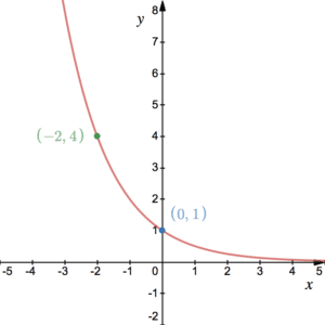
The graph of $y=a^x$ for $0< a< 1$ will have a shape like the graph above but will be reflected in the $y$ -axis. This is because when you multiply a number less than 1 by itself, it becomes smaller.

The following table shows coordinates for the graph $y=0.5^x$ for $x$ taking integer values between -3 and 3:

x	-3	-2	-1	0	1	2	3
y	8	4	2	1	0.5	0.25	0.125

For any number $0<a<1$ , the graph will have the same shape as $y=0.5^x$ .

For $a=1$ , the graph of $y=a^x$ is the horizontal line $y=1$ . This is because you are calculating 1 to any power, which is always 1. For negative a, fractional powers become an issue and complex numbers need to be considered.

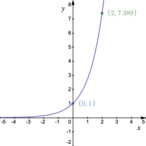
The diagram shows the graph of $y=e^{x}$ where $e$ , sometimes known as Euler’s number, is given by $e=2.718281828459$ … Since $e$ is positive and greater than 1, it looks very similar to the first graph above.

The number $e$ is special because everywhere on this graph, the gradient is the same as the $y$ -coordinate. See differentiating $e$ to the $x$ .

Logarithmic Graphs

As well as exponential graphs, there are logarithmic graphs. $\log_a(x)$ is considered to be the inverse of $a^x$ – see more on logs. It follows that $\log_a(x)$ (blue solid line) is the inverse of $a^x$ (red dotted line) and so their graphs are reflections of each other in the line $y=x$ (green dotted line). Since $\log_a(x)$ and $a^x$ are mathematical inverses we have that $\log_a\left(a^x\right)=a^{\log_a(x)}=x$ .
Specifically, the natural logarithm is the logarithm that corresponds to $e$ . That is, given an equation of the form $y=e^{x}$ , it can be said that $x=\log_e(y)$ . Since $e$ is a special number, log to the base $e$ has its own name. That is, it is the natural logarithm and often called $\ln$ so $x=\log_e(y)$ is more often written as $x=\ln(y)$ .

$\ln(x)$ and $e^x$ are mathematical inverses and we have that $\ln\left(e^x\right)=e^{\ln(x)}=x$ . Notice that $\log_a$ for any positive $a$ (including $\ln$ ) cannot be evaluated for negative $x$ – see more on logs.

Estimating Parameters

Estimating Parameters for $y=ax^n$

Consider the equation $y=ax^n$ . Note that, according to BIDMAS, this is $x$ to the power of $n$ , then multiplied by $a$ . This is a stretch to a standard polynomial curve – see Curve Sketching. Given this relationship and a dataset that approximately fits it, it is possible to estimate the parameters $a$ and $n$ . First consider what happens when logging both sides:

exponential graphs

$\begin{array}{lll}\log(y)&=&\log(ax^n)\\\Longrightarrow \log(y)&=&\log(a)+\log(x^n)\\\Longrightarrow \log(y)&=&\log(a)+n\log(x)\end{array}$

Note that the bases are missing this is true for any base (provided the same base is used for both). In the same way that you can plot y against $x$ , it is possible to plot $\log(y)$ against $\log(x)$ . Recall that, in the equation $y=mx+c$ , $m$ is the gradient and $c$ is the $y$ -intercept. In addition, we can write $\log(y)$ as $n\log(x)+\log(a)$ and so, in the plot of $\log(y)$ against $\log(x)$ , $n$ is the gradient and $\log(a)$ is the $y$ -intercept.

Estimating Parameters for $y=kb^x$

Now consider the equation $y=kb^x$ . Like the above, this is an exponential curve, provided $b$ is positive. Similarly to before, given a dataset or similar, we could estimate the parameters $b$ and $k$ . Taking logs:

exponential graphs

$\begin{array}{lll}\log(y)&=&\log(kb^x)\\\Longrightarrow \log(y)&=&\log(k)+\log(b^x)\\\Longrightarrow \log(y)&=&\log(k)+x\log(b)\end{array}$

It follows that $\log(y)$ can be written as $\log(b)x+\log(k)$ and so, this time, in the plot of $\log(y)$ against $x$ , $\log(b)$ is the gradient and $\log(k)$ is the $y$ -intercept.

Examples

The following table follows the relationship $y=ax^n$ where the $y$ values are given to one decimal place. By plotting $\log(y)$ against $\log(x)$ , estimate the parameters $a$ and $n$ to 1 decimal place.

x	2	3	4	5
y	26.4	104.7	278.6	594.9

Solution:

Logs of the $x$ and $y$ values can be calculated as follows:

log(x)	0.301	0.477	0.602	0.699
log(y)	1.42	2.02	2.44	2.77

Note that log without a specified base is usually log base 10. Plotting $\log(y)$ against $\log(x)$ , we can see a straight line that has a gradient of approximately 3.4 and a $y$ -intercept of approximately 0.4. It follows that $n=3.4$ and $a=10^{0.4}=2.5$ . Hence, the relationship between $x$ and $y$ as given by these points is approximately $y=2.5x^{3.4}$ .

Sample Edexcel Exam Question 14:

exponential graphs

Open Sample Exam Question in New Window

Solution:

Open Solutions in New Window

Extra Resources

https://www.youtube.com/watch?v=q9DhlR43P7A

Graphing a Logarithm – Made Easy! (https://www.youtube.com/watch?v=q9DhlR43P7A)

Graphing Logarithmic Functions

AS Maths Exponential & Logs

A2 Maths Exponentials & Logarithms

Return To The Maths Index

A-Level Mathematics

About

StudyWell is a website for students studying A-Level Maths (or equivalent. course). We have lots of resources including A-Level content delivered in manageable bite-size pieces, practice papers, past papers, questions by topic, worksheets, hints, tips, advice and much, much more.

Edexcel

Maths Pages

Useful Websites

Legal

Account